Original post is here: eklausmeier.goip.de
This post recaps the paper from Aaron J. Owens and D.L. Filkin from 1989: Efficient Training of the Back Propagation Network by Solving a System of Stiff Ordinary Differential Equations.
1. Neural network. Below is a single "neuron":
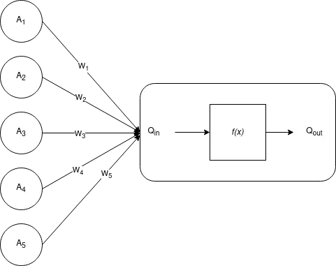
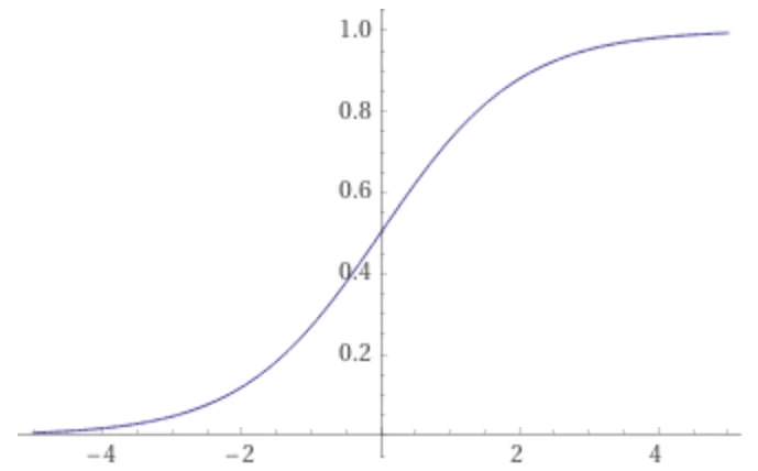
Input to node $Q$ is given in $A_i\in\mathbb{R}$, weights $W_i\in\mathbb{R}$, then node $Q$ computes $$ Q_{\hbox{in}} = \sum_i W_i A_i. $$ Output from node $Q$ is $$ Q_{\hbox{out}} = f(Q_{\hbox{in}})a. $$ The semilinear function $f(x)$, sometimes called "squashing function", is an increasing function of $x$ that has a limited range of output values. A commonly used squashing function is the sigmoid $$ f(x) = {1\over 1+\exp(-(x+\phi))}, $$ $\phi$ is called the threshold of the node. The squashing function has limits $0<f(x)<1$, which guarantees that the output of node $Q$ is limited to the range $0<Q_{\hbox{out}}<1$, regardless of the value $Q_{\hbox{in}}$. It looks like this, from Wolfram Alpha, for $\phi=0$.
Derivative of $f$ is $$ {df(x)\over dx} = \left(f(x)\right)^2 \exp(-(x+\phi)) = \left( 1 - f(x) \right). $$ Error from output $Q_{\hbox{out}}$ versus desired output $Y$ is $$ E := \left( Y - Q_{\hbox{out}} \right)^2. $$
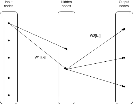
Multiple "neurons" from above can be stacked together. All nodes, which are not directly connected to input or output, are called "hidden layers". Below is a three-layer neural network.
2. Gradient descent. To change the weights $W_i$ via the method of steepest descent, find the gradient of $E$ with respect to $W_i$ and then change $W_i$ to move $E$ toward smaller values. Thus change according $$ \Delta W_i = -{dE\over dW_i}. \tag1 $$ Applying the chain rule and using above squashing function $f$ gives $$ \Delta W_i = 2 (Y-Q_{\hbox{out}}) Q_{\hbox{out}} (1 - Q_{\hbox{out}}) A_i. \tag2 $$ The weights are initialized to small random values. The weights are now changed according below rule: $$ W^{\nu+1} = W^\nu + \eta \Delta W^\nu + \alpha(W^\nu-W^{\nu-1}). \tag3 $$ Both $\eta$ and $\alpha$ are adjustable parameters and problem dependent. Typically with magnitudes smaller unity. Parameter $\alpha$ is called "momentum", parameter $\eta$ is called "training rate".
3. Stiff training. The authors, Owens+Filkin, were impressed by the similarities between temporal history of the weight changes and those of ordinary differential equations that are stiff. In place of the discrete equation (1), the weights $W_i$ are now to be considered functions of time. To change the weights so that the squared predition error $E$ decreases monotonically with time, the weights are required to move in the direction of gradient descent. Thus the discrete equation (1) is replaced with the ordinary differential equation (ODE) $$ {dW_i\over dt} = -{dE\over dW_i}. $$ Using the schematic equation $$ {dW_i\over dt} = \Delta W_i, \tag4 $$ where $\Delta W_i$ represents the weight changes given in (2). There is one ODE for each adjustable weight $W_i$, and the right-hand sides are nonlinear functions of all weights. Comparing equations (3) and (4) shows that each unit of time $t$ in our differential equations corresponds to one presentation of the training set in the conventional algorithm, with a training rate $\eta=1$.
The Hessian matrix $$ H_{ij} = -{\partial^2 E\over\partial W_i\partial W_j} $$ is the Jacobian matrix for the differential equation. All explicit numerical solution schemes have a limiting step size for stiff stability, which is proportional to $1/\Lambda$, where $\Lambda$ is the largest eigenvalue of the Hessian matrix.
Modern stiff differential equation solvers are A-stable, so that the stability of the numerical solution is not limited by the computational stepsize taken.
The tolerance used for the numeric solver can be quite loose. Owens+Filkin chose $10^{-2}$, i.e., 1%. Owens+Filkin provide below performance table.
| RMS error | Nonstiff / stiff | gradient descent / stiff |
|---|---|---|
| 10% | 1 | 1 |
| 5% | 2 | 4 |
| 2% | 5 | >20 |
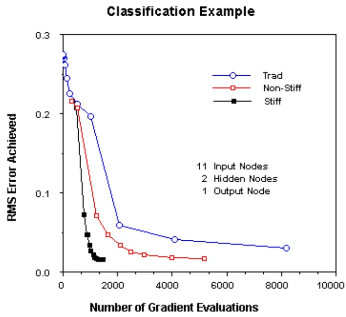
4. Classification and orientation. The results of Owens+Filkin (1989) have been confirmed by Alessio Tamburro (2019).
Fewer iterations or presentations of the data to the network are needed to reach optimal performance. [Though] The use of a ODE solver requires significantly greater computation time.
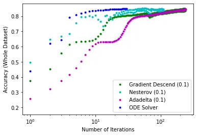
It remains remarkable that stiff ODE solvers are not used more often in the setting of neural networks. See Reply to: Neural Network Back-Propagation Revisited with Ordinary Differential Equations. The main points were:
- Tolerances employed were very strict, too strict in my opinion, especially during initial integration
- Completely incomprehensible that zvode, the "Complex-valued Variable-coefficient Ordinary Differential Equation solver" was used
- A "switching" solver, i.e., one that can automatically switch between stiff and non-stiff would likely improve the results
Currently used neural networks have quite a number of weights.
| Neural network | number of weights | reference |
|---|---|---|
| LLaMa | 13 × 109 | Wikipedia |
| ChatGPT-3 | 175 × 109 | Wikipedia |
| ChatGPT-4 | 1000 × 109 | The decoder |
Added 09-Jul-2023: Nice overview of some activation functions is here Activation Functions in Neural Networks. PyTorch's activation functions are listed here. Activation function in Twitter format as below. A separate discussion of the so called "rectifier function" is in Wikipedia. Also see Activation Functions: Sigmoid vs Tanh.
[twitter] https://twitter.com/akshay_pachaar/status/1672220488133939200 [/twitter]